How to Create Line Charts in Matplotlib Python?

Line charts
A Line chart shows how a variable’s value changes over time. The x-axis represents the time frame, such as months or years. The y-axis represents the value we are interested in measuring, like revenue or the number of visitors to a website. We can also create multiple line charts to compare related groups over time, such as the population of India, China, and the US in the past 20 years.
Read data
We will use the Pandas library for data manipulation and analysis. Let’s import it and read a dataset using the `read_csv()` function. We will also convert the `Date` column to `datetime` using the `parse_dates` parameter. You can download the data from here - matplotlib-python-book
# silence warnings
import warnings

warnings.filterwarnings("ignore")

# import pandas
import pandas as pd

# read the data into pandas DataFrame
nvidia = pd.read_csv("../data/NVDA.csv", parse_dates=["Date"])
nvidia.head()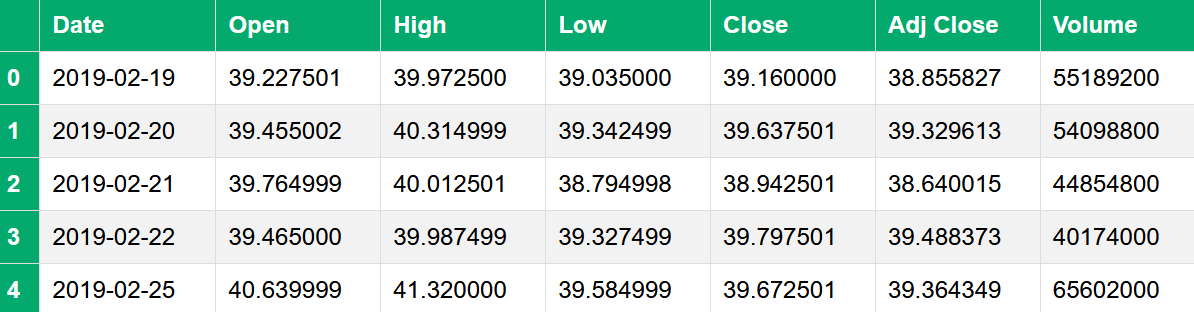
Create a Line chart
To create a line chart in Matplotlib, we use the plt.plot() function and the plt.show() function to show the figure.
Before creating any chart in Matplotlib, we must import the Matplotlib library first using `import matplotlib.pyplot as plt`. Let’s create a line chart with `Date` on the x-axis and `Adj Close` on the y-axis.
# import matplotlib library
import matplotlib.pyplot as plt

# create a line chart
plt.plot(nvidia["Date"], nvidia["Adj Close"])
plt.show()
Title and Axis labels
Let’s add a title to the plot using the plt.title() and x and y-axis labels using the plt.xlabel() and plt.ylabel() respectively.
# line chart with title and axis labels
plt.plot(nvidia["Date"], nvidia["Adj Close"])
plt.title("Nvidia Stock Prices (2019-2024)")
plt.xlabel("Year")
plt.ylabel("Adj Close Price")
plt.show()
We can see that the share price of Nvidia constantly went up from 2019-22, and then it started to go down between 2022-23. It then rose again and went very high at the beginning of 2024.
The reason for such a hike in Nvidia stock prices is the explosion of artificial intelligence and its revenue from selling `GPUs,` which are needed to train large machine learning models. Nvidia controls more than 95% of the GPU market.
Multiple line charts
We need to add another `plt.plot()` function to create multiple line charts on the same figure. This will instruct matplotlib to create another line with the same x and y-axis as the first figure.
Let’s read some more data for this.
# read data
netflix = pd.read_csv("../data/NFLX.csv", parse_dates=["Date"])
tesla = pd.read_csv("../data/TSLA.csv", parse_dates=["Date"])
We will create a line chart on the same plot for Nvidia, Netflix, and Tesla.
# create multiple line charts
plt.plot(nvidia["Date"], nvidia["Adj Close"])

plt.plot(netflix["Date"], netflix["Adj Close"])

plt.plot(tesla["Date"], tesla["Adj Close"])

plt.title("Stock Prices (2019-2024)")
plt.xlabel("Year")
plt.ylabel("Adj Close Price")
plt.show()
Legend
Although we plotted all the lines on the graph, which line corresponds to which company needs to be clarified. To solve this problem, we need to add a legend to the plot. First, we will add labels to each line and then use plt.legend() function to add a legend.
# multiple line charts with legend
plt.plot(nvidia["Date"], nvidia["Adj Close"], label="Nvidia")

plt.plot(netflix["Date"], netflix["Adj Close"], label="Netflix")

plt.plot(tesla["Date"], tesla["Adj Close"], label="Tesla")

plt.title("Stock Prices (2019-2024)")
plt.xlabel("Year")
plt.ylabel("Adj Close Price")
plt.legend()
plt.show()
Line style and color
We can apply our own line styles and colors instead of default ones. Use the `linestyle` and `color` parameters to change the line style and color.
# Line chart with custom line style and color
plt.plot(tesla["Date"], tesla["Adj Close"], label="Tesla", linestyle=":", color="blue")

plt.plot(
    nvidia["Date"],
    nvidia["Adj Close"],
    label="Nvidia",
    linestyle="--",
    color="seagreen",
)

plt.plot(
    netflix["Date"],
    netflix["Adj Close"],
    label="Netflix",
    linestyle="-.",
    color="crimson",
)

plt.title("Stock Prices (2019-2024)")
plt.xlabel("Year")
plt.ylabel("Adj Close Price")
plt.legend()
plt.show()
The plot with solid lines looked much better than this version. You can use many other parameters to change the appearance of a line chart; please refer to the document. line chart
Style sheets
Various style sheets are also available to change the appearance of your plots. You can list the styles available using the `plt.style.available` attribute. You can also see examples of them here - style sheets reference.
To add a style, use the `plt.style.use(‘stylesheet_name‘)`.
# Add a style sheet in matplotlib
plt.style.use("seaborn-v0_8-dark")

plt.plot(tesla["Date"], tesla["Adj Close"], label="Tesla", color="blue")

plt.plot(nvidia["Date"], nvidia["Adj Close"], label="Nvidia", color="seagreen")

plt.plot(netflix["Date"], netflix["Adj Close"], label="Netflix", color="crimson")

plt.title("Stock Prices (2019-2024)")
plt.xlabel("Year")
plt.ylabel("Adj Close Price")
plt.legend()
plt.show()
Figure size
To change the size of a figure, use the `figsize` parameter of the plt.figure() function. The `figsize` takes a tuple of (`width`, `height`) in inches.
# Change figure size
plt.figure(figsize=(7, 5))

plt.plot(tesla["Date"], tesla["Adj Close"], label="Tesla", color="blue")

plt.plot(nvidia["Date"], nvidia["Adj Close"], label="Nvidia", color="seagreen")

plt.plot(netflix["Date"], netflix["Adj Close"], label="Netflix", color="crimson")

plt.title("Stock Prices (2019-2024)")
plt.xlabel("Year")
plt.ylabel("Adj Close Price")
plt.legend()
plt.show()
Save a figure
To save a figure in matplotlib, use the `plt.savefig(‘filepath/image.png‘)` function before calling the `plt.show()` function. You can also use other image extensions like `jpeg,` `pdf,` etc.
plt.figure(figsize=(7, 5))

plt.plot(tesla["Date"], tesla["Adj Close"], label="Tesla", color="blue")

plt.plot(nvidia["Date"], nvidia["Adj Close"], label="Nvidia", color="seagreen")

plt.plot(netflix["Date"], netflix["Adj Close"], label="Netflix", color="crimson")

plt.title("Stock Prices (2019-2024)")
plt.xlabel("Year")
plt.ylabel("Adj Close Price")
plt.legend()
# save it in the image folder
plt.savefig("../images/stock_prices_2019_2024.png")
plt.show()
Exercise 2.1
Read the `marriage-age-2016.txt` in pandas with the sep=’\t’ parameter.
Use the same figure to create a line chart of men’s and women’s ages at marriage over time.
Create a new column, `age_diff,` by subtracting Women’s ages from Men’s ages at marriage.
Create a line chart showing age differences over time.
Summary
To create a Line chart in matplotlib, use the `plt.plot()` function.
Use `plt.title()` to add a title to the plot.
For x and y-axis labels, use `plt.xlabel()` and `plt.ylabel()`, respectively.
Multiple line charts can be added to the same figure by adding another plt.plot() function.
To add a legend, specify `label` for each line and then use `plt.legend()`.
Use `linestyle` and `color` to change line style and color.
To use style sheets in matplotlib, use `plt.style.use(‘stylesheet_name`)`.
Use `figsize` to change the figure size.
Use the `plt.savefig()` to save a figure.
Solution
Exercise 2.1
# ignore warnings
import warnings

warnings.filterwarnings("ignore")

# import libraries
import pandas as pd
import matplotlib.pyplot as plt

plt.style.use("seaborn-v0_8-dark")

# Read the marriage-age-2016.txt in pandas
marriage = pd.read_csv("../data/marriage-age-2016.txt", sep="\t")

# Create a new column age_diff
marriage["age_diff"] = marriage["Men"] - marriage["Women"]

# Line chart of men's and women's ages at marriage
plt.plot(marriage["Year"], marriage["Men"], label="Men", color="crimson")

plt.plot(marriage["Year"], marriage["Women"], label="Women", color="seagreen")

plt.title("Age at Marriage By Gender (1890 - 2016)")
plt.xlabel("Year")
plt.ylabel("Age at Marriage")
plt.legend()
plt.show()
We can see that for both men’s and women’s age at marriage dropped for a while then increased after 1980. There is an upward trend in People getting married late.
# Line chart of men's and women's age difference.
plt.plot(marriage["Year"], marriage["age_diff"], color="crimson")

plt.title("Age Difference at Marriage (1890 - 2016)")
plt.xlabel("Year")
plt.ylabel("Age difference at Marriage")
plt.show()
We can also see that the difference in age between men and women in marriage is dropping over time. More men and women are getting married to people of their age, and the age difference is reducing.
Pre-order
If you enjoyed this article and are looking for more insightful content, consider pre-ordering my upcoming book on matplotlib at a 40% discount, or subscribe to our newsletter below for free. Your support helps me continue to share valuable knowledge. Thank you for reading.